In Vivo Validation of an In Situ Calibration Bead as a Reference for Backscatter Coefficient Computation

Introduction

Backscatter coefficient (BSC) represents the quantity of backscattered signal coming from a volume of soft tissue. It is linked to the density, shape and size of scatterers in it and can therefore provide valuable information about its structure. The BSC gives quantitative results that are system and operator independent. It has shown potential for liver steatosis diagnosis as well as tumor treatment monitoring. This study focuses on the latter case. The most commonly used method to estimate the BSC is based on the reference phantom method (RPM) which has demonstrated great results but suffers from inherent problems. The main contribution of this study is the in vivo validation of an in situ calibration bead as an alternative to the RPM. This review will first introduce the RPM and its limitations. Next, the paper’s methodology and results will be presented, followed by a discussion of its findings.

The reference phantom method (RPM)

The RPM method uses the backscattered RF data from the sample, a tumor in this case:

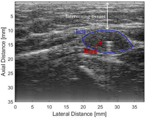
B-mode image of a tumor highlighted in blue, white arrow depicts the intervening tissues (pork belly), red arrow shows the position of the calibration bead. Modified from the original paper.

The power spectrum \(W(f)\) of the signal coming from the region of interest (ROI) is written as:

\[W(f) = H(f)D(f,x)A(f,x)T(f,x)S(f,x),\]

where \(H(f)\) is the system impulse response, \(D(f,x)\) is the diffraction factor that depends on the position \(x\), \(A(f,x)\) and \(T(f,x)\) represent the attenuation and transmission losses caused by tissues, \(S(f,x)\) is the backscattering function describing the underlying tissues. The whole point of the RPM is to isolate this last part by normalizing \(W(f)\) by the power spectrum \(W_{ref}(f)\) of a reference phantom measured under the same conditions. The estimated BSC \(\sigma(f,x)\) is:

\[\sigma(f,x) = \frac{W(f,x) A(f,x) T(f,x)}{W_{ref}(f,x) A_{ref}(f,x) T_{ref}(f,x)}\sigma_{ref}(f,x)\]

By doing so, the system impulse response and the diffraction factor cancel out. The BSC of the reference is known either by using a theoretical model or by performing a calibration. Since the travel path of the wave is not the same for the sample and the reference phantom, it is necessary to compensate for the difference in attenuation and transmission. Attenuation and transmission are easy to estimate in the reference phantom but can be difficult to determine in the intervening tissues. Errors in this compensation will result in a higher variance and bias when computing \(\sigma(f,x)\).

Proposed method

The bead method

The idea behind the paper is to work around the limitations of the RPM by directly placing a titanium bead inside the ROI and using its reflected signals as the reference measurement. This methodology ensures that the \(W(f,x)\) and \(W_{bead}(f,x)\) share approximately the same transmission and attenuation loss. The BSC formula becomes:

\[\sigma(f,x) = \frac{W(f,x)}{W_{bead}(f,x)}\sigma_{bead}(f,x).\]

In this new formula, the estimation of \(A(f,x)\) and \(T(f,x)\) is no longer necessary. The authors hypothesize that this will reduce the variance and bias of the BSC estimates.

A 2 mm titanium bead was used for the in vivo measurements. Its BSC was calibrated to use it as a reference. For this purpose, they embedded the bead inside a tissue mimicking phantom with a known BSC. Then, they computed the power spectrum of signals reflected by the bead and by the phantom at the same depth. Finally, the RPM gave the BSC of the bead.

In vivo measurements

21 rabbits with injected mammary tumors were scanned. The bead was injected 3 days before the experiments to avoid blood pooling effects. Data were acquired using a L14-5/38 linear probe. A free-hand scan of the tumor was performed to obtain a volumetric scan of the tumor.

To simulate the effect of the intervening tissues, the acquisitions were made with and without a pork belly between the probe and the tumor. This layer was ~1.5-2 cm thick.

The position of the bead was found by doing a cross-correlation between the B-mode image and a bead spread function. To ensure that they computed the spectrum on the maximum bead signal, as in the calibration step, they interpolated the volume in both lateral and elevational directions, as illustrated in:

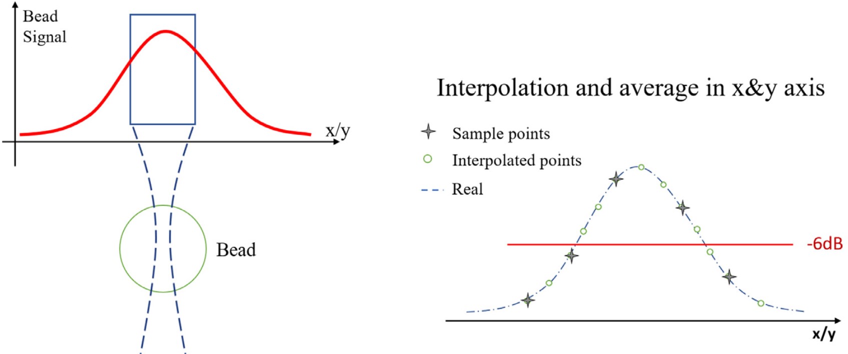
Signal energy decreases from the center of the bead. Interpolation of the data points helps recover the maximum signal.

Resuts

The BSC was computed in 4 cases:

• A) With the RPM and no pork belly.
• B) With the bead method and no pork belly.
• C) With the RPM and pork belly.
• D) With the bead method and pork belly.

Case A is considered the true measurement and serves as a reference for error estimation.

Here are the results for the mean BSC:

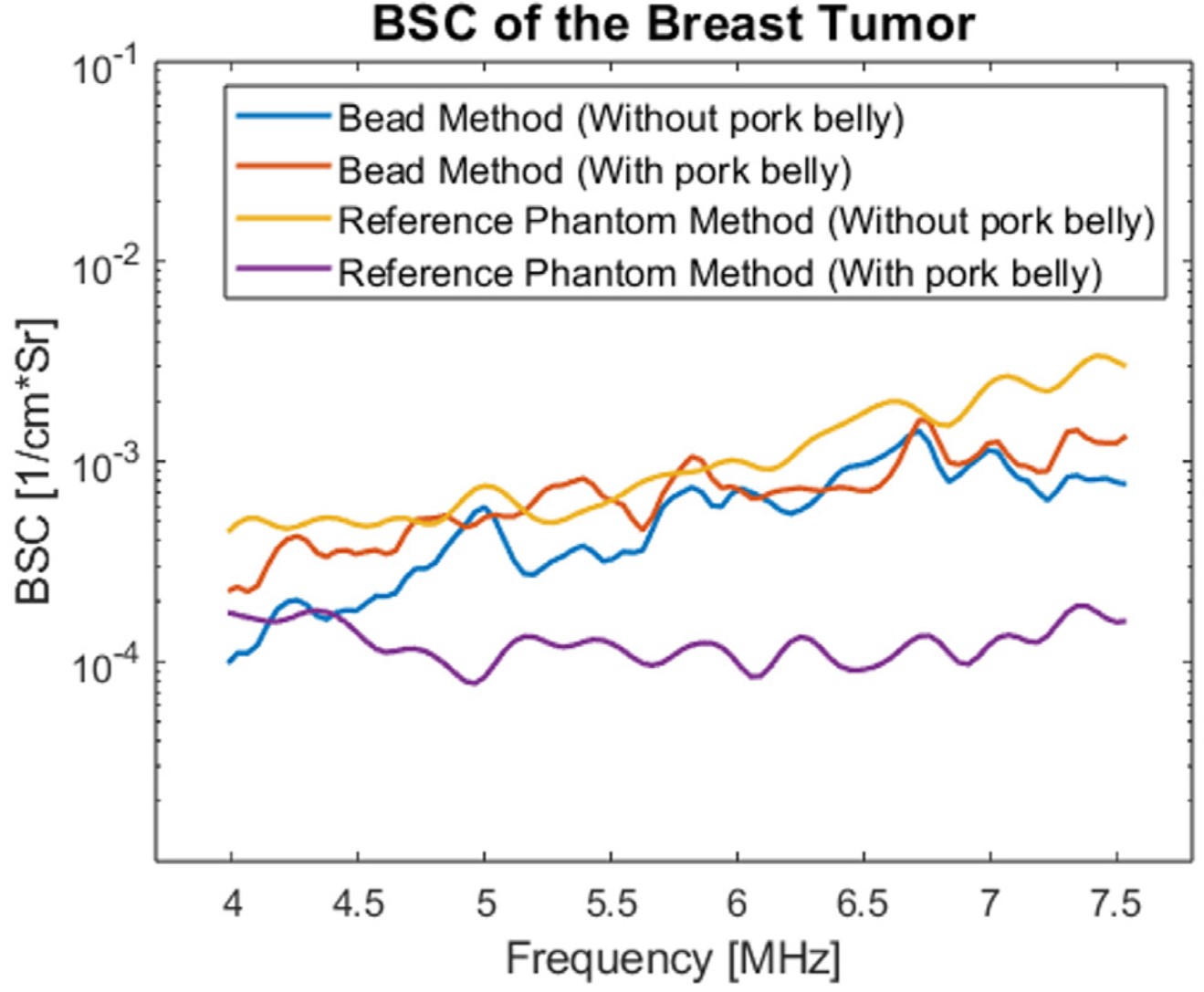
Mean BSC of the tumor using both the reference and the bead method.

The bead without pork belly, case B, gave results comparable to case A. This shows the accuracy of the bead method. The addition of pork belly had a strong impact on the results of the RPM. If the attenuation and transmission loss were perfectly compensated the intervening tissues should have no impact on the BSC. The bead method was minimally affected.

To further the analysis, they computed the equivalent scatterer diameter (ESD) and the effective acoustic concentration (EAC) by fitting a Gaussian model to the BSC curve. These parameters are helpful because they can bring some physical meaning to the BSC estimation. The next figure shows the mapping of the ESD in the same tumor in the 4 cases:

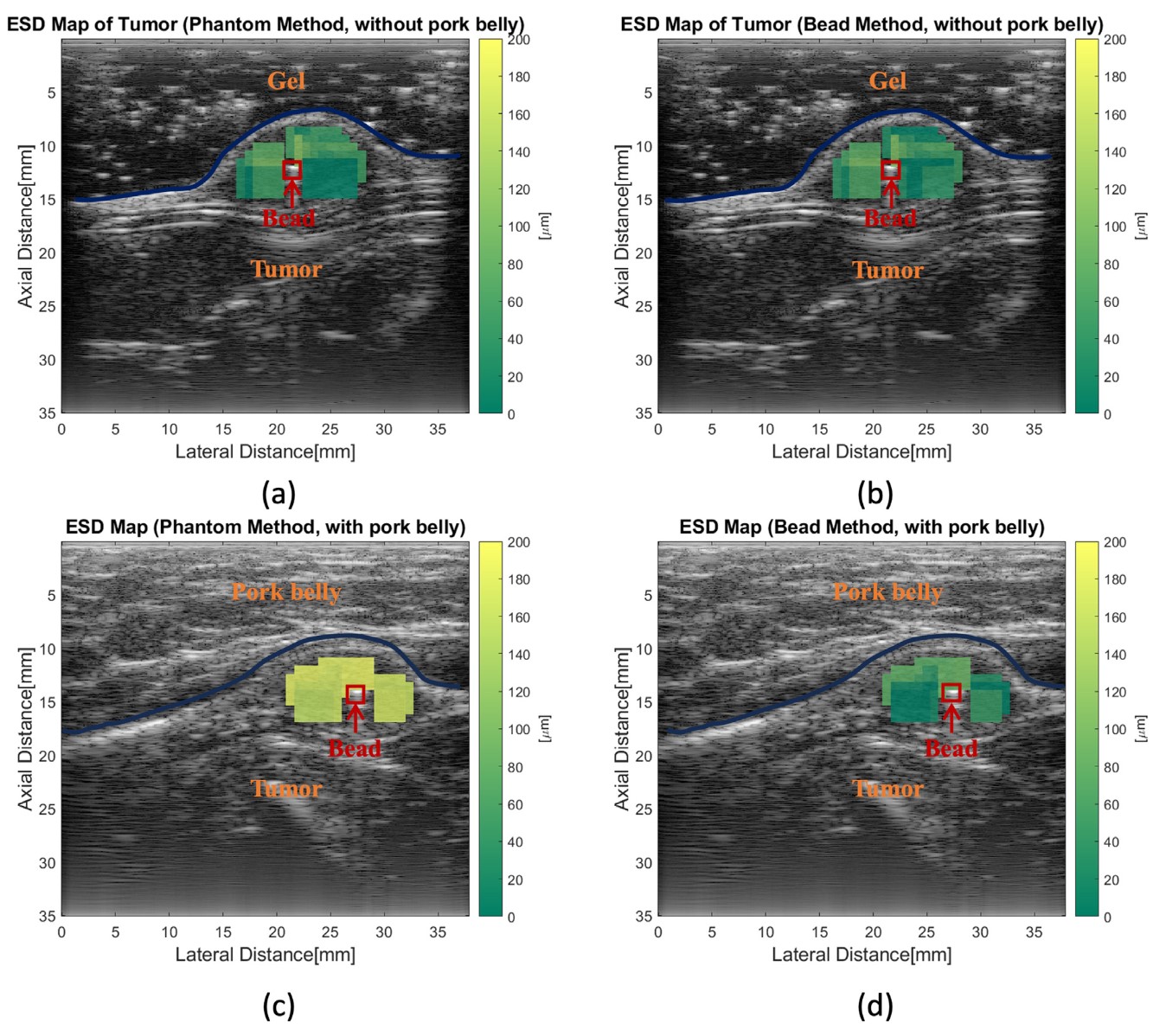
Equivalent scatterer diameter of a tumor using the reference phantom method and the bead method, with and without pork belly.

The estimations without pork belly were in good agreement. However, when the pork belly is added, a clear shift is seen in the ESD map of the RPM method. No apparent shift can be seen in the bead method.

They also computed the absolute difference of the ESD and EAC between the cases B, C, D and case A.

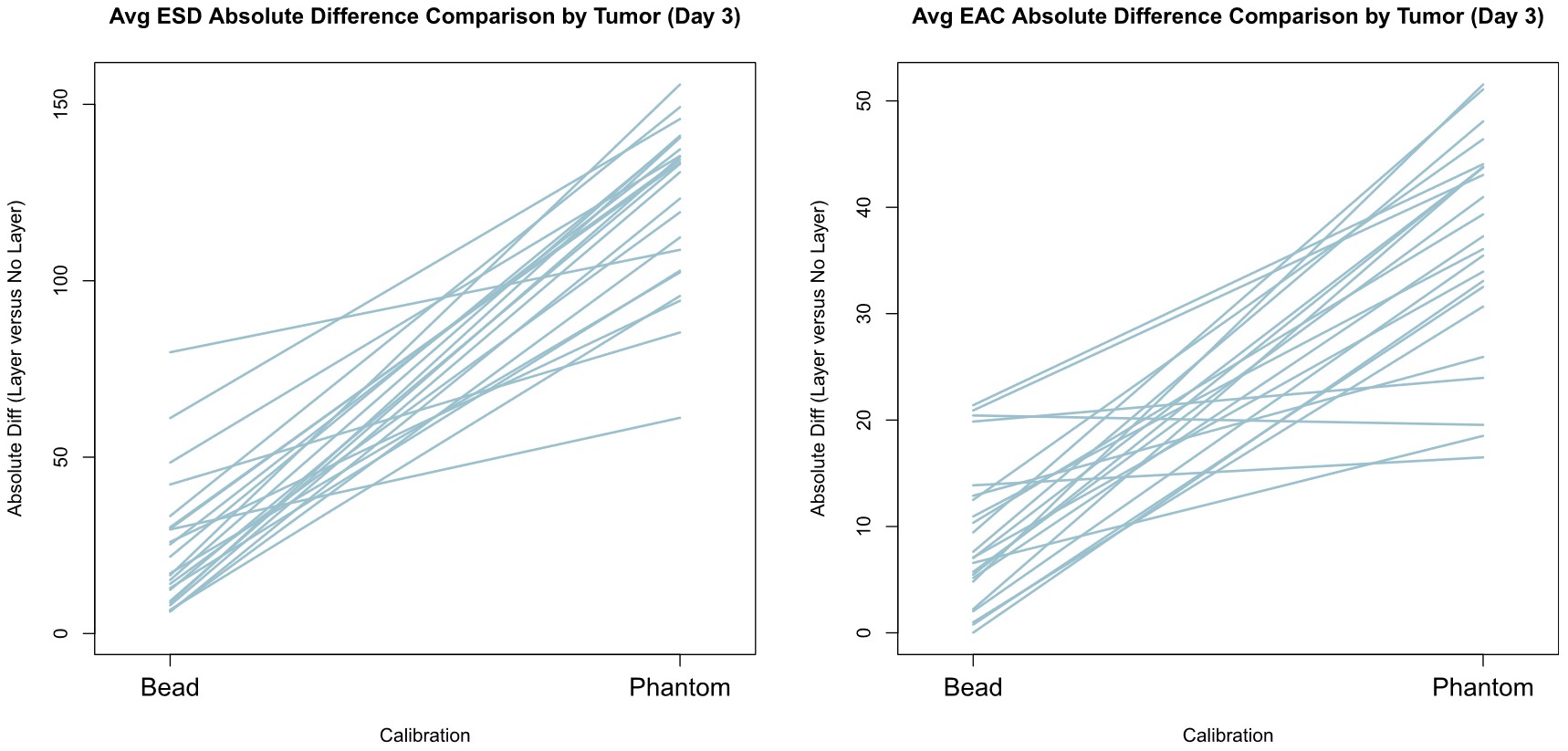
Mean absolute difference of the ESD and EAC was computed in case B, C, D and compared to case A. Each line represents a different tumor.

In each tumor, the error was higher for the RPM than for the bead method.

Results show that the bead method can give results equivalent to the RPM but with a greater consistency with intervening tissues.

Discussion

This article is not the first to bring up the idea of using an in situ calibration for BSC computation. However, it is the first one to do a comparison with the RPM on in vivo data. It provides a solution to the long-lasting problem of compensating the attenuation and transmission loss inside soft tissues. The results are interesting and encouraging, however, some limitations are present.

• In practice, the insertion of a metal bead in a human patient may discourage the use of this method, as it is no longer non-invasive. The authors respond that some clips and markers are already in use for cancer imaging and during therapy. Moreover, 2 mm gold beads have been approved by the U.S. Food and Drug Administration to be used in human patients. The use of a calibration bead should not be a barrier to the application of the proposed method.

• The authors also showed that the bead method has higher error when the signal to noise ratio (SNR) is low. To mitigate this, it is worth noting that this issue is common in most ultrasound techniques.

• The authors didn’t specify how they estimated the attenuation and transmission loss of the pork belly. Perhaps a more advanced method could have reduced the error of the RPM when adding the pork belly to the measurements.

• It can be seen on the ESD map that no estimation is made under the bead. In fact, the reverberation and strong reflectivity of the bead create a shadow zone where it is impossible to estimate the BSC.

• The estimations are not always at the same depth as the bead. For example, in the ESD map, this difference is not taken into account in the bead method and may introduce errors in the estimation.

• From the reviewer’s understanding, the formula of \(\sigma(f,x)\) given in the paper is inconsistent. In order to properly compensate for the attenuation and transmission loss, \(A_{ref}(f,x)\), \(T_{ref}(f,x)\) should be in the numerator and \(A(f,x)\), \(T(f,x)\) in the denominator.